Harun Legoz

Introduction

There are many ways to build an ETL process in on-premise, but there's no simple way or a more comprehensive product in Azure. One option is to adopt a product built for another purpose and try to make use of it, which quite often fails miserably (like Azure Data Lake Analytics). Another option is to develop something from scratch, which requires world-class level design and development process. Most of these ETL requirements surface within another project, which possibly doesn't have time or resources to accomplish something like that.

Recently, Microsoft has been investing a lot on both Azure Data Factory and Azure Databricks. Databricks lets you process data with managed Spark clusters through the use of data frames. It's a fantastic tool, but it requires a good knowledge of distributed computing, parallelization, Python or Scala. Once you grasp the idea, it propels you forward like a photon torpedo. However, it's a pain to learn.

Azure Data Factory, on the other hand, has many connectivity features but not enough transformation capabilities. If the data is already prepared or requires minimal touch, you can use ADF to transport your data, add conditional flows, call external sources, etc. If you need something more, not helpful enough. At least it wasn't until Microsoft released its next trick in its sleeves to the public.

Azure Data Flow is an addition to Data Factory, backed by Azure Databricks. It allows you to create data flows to manipulate, join, separate, aggregate your data visually, and then runs it on Azure Databricks to create your result. Everything you do with Azure Data Flow is converted to Spark code and executed on your clusters, which makes them fast, resilient, distributed and structured.

It provides the following activities:

• New Branch
• Join
• Conditional Split
• Union
• Lookup
• Derived Column
• Aggregate
• Surrogate Key
• Pivot
• Unpivot
• Window
• Exists
• Select
• Filter
• Sort
• Extend
• Table of Contents

To achieve an ETL pipeline, you compose a data flow with the activities above. A sample flow can contain a Source (which points to a file in blob storage), a Filter (which filters the source based on a condition), and a Target (which leads to another file in blob storage).

It has many great features, but it also has its limitations. At the moment, you can only specify file-based sources (Blob and Data Lake Store) and Azure SQL Database. Everything else, you can put a copy activity on your Data Factory pipeline before you call Data Flow, which will allow you to query your source, output its results to the blob, then execute the Data Flow on this file. Similarly, that's also what you need to do if you want to write to other sinks.

Let's carry on with our experiment.

Objectives

For our experiment, we'll use a data file that contains the football match results in England, starting from 1888. The data file is available here and is around 14MB.

We'll load the data into our storage account and then calculate three different outputs from that:

• Total matches won, lost and drawn by each team, for each season and division
• Standings for each season and division
• Top 10 teams with most championships

The objective of our experiment is to prove that Data Flow and Data Factory;

• Can create complex data processing pipelines
• Is easy to develop, deploy, orchestrate and use
• Is easy to debug and trace issues

Implementation

Source code for this example is can be downloaded below. It includes the Data Factory files as well as the example csv file, which you need to upload it to a blob storage and configure your linked services.

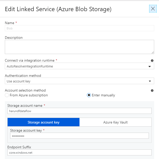
We start with loading our CSV file into blob storage that we can access in Data Factory. For this, you'll need to create a Blob Storage and then create a linked service for it:

First Example: Team Analytics

Then, we can continue to create our Datasets. For this experiment, we'll need 4 datasets: MatchesCsv (our input file), AnalyticsCsv (for team analytics), SeasonStandingsCsv (for each season standings) and MostChampionsCsv (for showing top champions). All four is available with the source code of this article, but all of them are CSV files that have headers enabled. The only difference is the output files doesn't have an output file name; only folders. This is a requirement from Data Flow (actually, Spark) so that it would create files per partition under this path.

Next thing on our list is to create our Data Flow. Data Flow is built on a few concepts:

• A data flow needs to read data from a source and write to a sink. At the moment, it can read files from Blob and Data Lake, as well as the Azure SQL Database. I've only experimented with Blob files but will try to do with SQL.
• It's essentially creating a Spark Data Frame and pushes it through your pipeline. You can look them up if you want to understand how it works under the hood.
• You can create streams from the same source or any activity. After you add an activity, click the plus sign again and select New Branch. This way, you don't have to recalculate everything up until that point, and Spark optimizes this pretty well.
• Flows cannot work on their own; they need to be put into a pipeline.
• Flows are reusable; you can reuse and chain them in many pipelines.
• In private preview, you could also define your custom activities by uploading Jar files as external dependencies, but they removed it on the public preview.

Enough with the advertisement, let's get our hands dirty. We'll start with our first case: Calculating the team analytics for each season and division. To do this, we'll create a flow that'll follow these steps;

• The dataset shows match results, so it has a Home and an Away team column. To create team-based statistics, we best build a file structure with a single column named Team.
• We do this by separating our source stream into two: Home Scores and Away Scores. It's a Select activity that formats the Home column as Team for Home Scores, Away for the Away Scores.
• Then, we need to add three columns based on the Result column (which has three values: 'H' for a Home win, 'A' for an Away win, 'D' for a Draw): Winner, Loser and Draw. These are boolean fields and checks if the team is a winner, a loser, or it's a draw. We'll base our statistics on these. For the Home team, Winner is when Result equals 'H' and Loser is when Result equals 'A'. For Away teams, it's the other way. We'll achieve this using Derived Column activity.
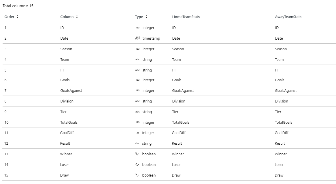
• Then we use Union to combine these two datasets and form a dataset we can run stats on AllStats. It looks like this:

Now, here's what we want to create as an output. Just like any good SQL statement, we'll achieve this by using Group By and then running aggregations on it. We'll do that using the Aggregate activity, named TeamAnalytics), and configuring it like below:

• Group By
  • Season
  • Division
  • Team
• Aggregations
  • Wins: countIf(equals(Winner, true()))
  • Loses: countIf(equals(Loser, true()))
  • Draws: countIf(equals(Draw, true()))
  • GamesPlayed: count(ID)
  • GoalsScored: sum(Goals)
  • GoalsAgainst: sum(GoalsAgainst)
  • GoalDifference: sum(Goals) - sum(GoalsAgainst)
  • Points: (3 * countIf(equals(Winner, true()))) + countIf(equals(Draw, true()))

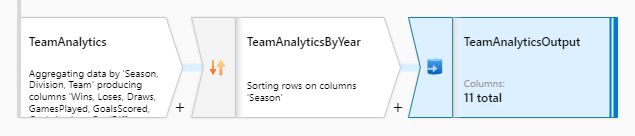
When executed, this code will run aggregations and create statistics output. Next step is to dump this into the blob storage; but first, we order it using the Sort activity (by Season, desc) and set its partitioning to Key. This will create a separate file per season so that we can have smaller and more organized files. Unfortunately, I have no idea how to give a meaningful name to the file names at this point, but I'm sure there'll be a way in the future. Now, we can use Sink activity to dump our contents into AnalyticsCsv dataset.

Next: Season Standings

Now that we know how each team performed on each season and division, we can create more sophisticated reports. Next one is to create each team's standings on their season and division. We'll do this by again grouping by teams and giving them a ranking by their position in the league, which will be based on their points in descending order. Now, I know that we have a crude point calculation (3 points for winnings and 1 point for draws) and we have neither overall nor individual goal difference in the calculation, but hey, football's already too much complicated these days.

We branch the TeamAnalytics activity and add a Window to the new stream. The Window looks like a very complicated activity, and it is, but we already know something similar in the SQL world for that: Things like ROW_NUMBER() OVER (Count DESC). The Window does the same thing, better explained by its help graphic:

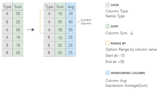
The main idea is to group and sort rows and create windows for each of them; then calculate aggregations on each window. It works quite similar to its SQL equivalent, and it's as much powerful. We'll use it to create groups by Season and Division, then sort by Points in descending order and calculate row number for each row:

• Over
  • Season
  • Division
• Sort
  • Points, DESC
• Range By
  • Range by current row offset
  • Unbounded
• Window Columns
  • Ranking: rowNumber()

We'll then proceed and dump this into another CSV dataset of ours, SeasonStandingsCsv.

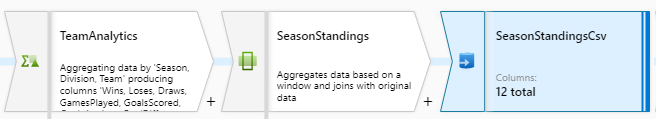
Next: Top 10 Most Champions

Our next step is to create a list of top 10 teams with most championships. To do that, we'll branch SeasonStandings and apply a series of transformation on it.

• Filter: To get only the champions from each season and division.
  • equals(Ranking, 1)
• Aggregate: To calculate championship count for each team
  • Group By:
    • Team
  • Aggregates:
    • Count: count()
• Window: To calculate row number by sorting the entire list descending on Count
  • Over
    • 0*Count: ID
  • Sort
    • Count: ASC
    • Team: DESC
  • Range By
    • Range by current row offset
    • Unbounded
  • Window Columns
    • No: rowNumber()
• Filter: To get top 10 rows based on No row number column
  • lesserOrEqual(No, 10)
  • Optimize: Single partition

You see that it's unusually long and complicated flow to get top 10 rows. Usually, after the aggregate activity, we should've been able to use Filter to get the top 10 rows directly. However, Data Flows Filter activity does not yet support Top N functionality, yet, so we had to improvise. The workaround is to put all the records into the same window (0*Count which will result as 0 in ID column), sort by count in desc, then add row number as a column. The trick here is to put everything in a single window. Otherwise, it would restart the row number for each window. I know, it's a workaround, but hey, life is a big workaround to death anyway.

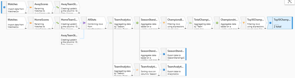
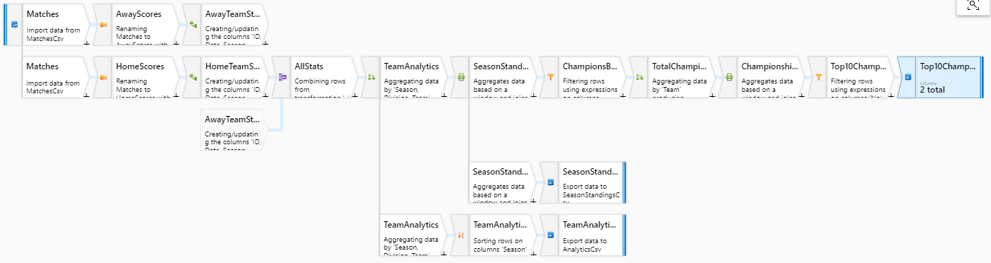
After these, we can safely dump our result set into our MostChampionsCsv dataset. Here's how our calculation branch looks like:

And finally, here's our grand result with three different sinks and many streams:

Conclusion

I have categorized my comments on Data Flows below but long story short, it looks like a promising product. It handled complex scenarios well, and Microsoft seems to be investing a lot on it. If it happens to be a success, we'll have an excellent tool to design our ETL processes on Azure, without the need of any third party tools.

Capabilities

• Positive
  • I found the Data Flow quite powerful and capable of creating complex data flows. Especially being able to develop team rankings by seasons with the help of Windows Activity shows that most of our data processing use cases can quickly be addressed with Data Flows.
  • There's a good collection of activities available for data transformation. It covers most scenarios; if not, you can always enrich it with other Data Factory (not Data Flow) capabilities, like Azure Function calls.
  • It looks like Microsoft is investing a lot on Data Factory and Data Flows. On data set creation page, it says it'll support most of the sources of Data Factory in Data Flows as well. This is good, means that we can always query the source directly with Data Flow and won't be bothered to download the data into a CSV first and then process it.
  • Considering that Data Flows live inside the Data Factory Pipelines, it benefits from all features it provides. You can trigger a pipeline with an event, which can connect to a source, transform it, and then dump the results somewhere else. It also uses Data Factory's monitoring and tracing capabilities, which is quite good. It even shows Data Flow runs in a diagram, so you can see how many rows have been processed by each activity.
  • The Window activity is quite powerful when creating group based calculations on the data (like rowNumber, rank, etc.).
  • Creating data streams and processing data through that with activities makes your flow easily readable, processable, and diagnosable.
  • To develop and see your activities' outputs instantly, there's a feature called Debug Mode. It attaches your flow to an interactive Databricks cluster and lets you click on activities, change them and see the result immediately without the need of deploying any flow or pipeline and then running it.
  • Even though it's still in preview, Data Flows are quite stable. Keep in mind that even if it has a Go-Live license, things can always change until GA.
  • Also thinking that the flow definition is just a JSON file, it makes it possible to parse it and use it in the data catalog. We can parse these transformation rules to calculate data lineage reports in the future.
• Negative
  • No "Top N Rows" support in Filter activity yet. Not essential, but annoying.
  • In the private preview, we were able to create a Databricks cluster and link it in Data Factory. This allowed us to control and maintain our clusters if needed, as well as to keep them up or down at specific times. Now in public preview, we cannot specify our Databricks. , and it spawns a new cluster every time you start a job. Considering that an average cluster wakes up around in 5 minutes, it increases the job run times significantly, even for small jobs.
  • By removing the Databricks linked service, they also removed the support for custom code (Extend activity). It wasn't a necessary capability, but knowing that it was there was a comfort for future complex scenarios. Now that it's gone, we cannot create custom Spark functions anymore.
  • Another consideration over auto-managed clusters is the data security part. It's not clear yet how and where Data Factory manages these clusters. There's no documentation around it yet, so it's a future task.

Development Environment

• Positive
  • Even though you are developing through the Azure Portal, not from your regular IDE, it's still an excellent experience. The Data Factory portal is quite reliable and works as powerful as an IDE.
  • From the portal, you can download the latest version of your pipelines, datasets, and dataflows as JSON and put it into your source control later. This requires the development environment to be shared by the developers, but with proper planning and multiple dev environments, I'm sure that won't be an issue.
  • Data Factory also has source control integration directly through its portal. You can hook it up to a Git repo, create branches, load your pipelines and flows, commit your changes, deploy them, create PRs, etc. It makes a good IDE experience on the portal.
  • You can also download the ARM template and incorporate it with your source control easily. It also allows you to import the ARM template, which can be handy in some cases.
  • Each pipeline, dataset, and flow has a JSON code which you can see and download. Then, with the Data Factory API, you can deploy them into any Data Factory.
• Negative
  • One thing I didn't like was when you add a source, point it to a dataset and import its schema into your source, it just loses the data types as well as the formats. This is annoying and requires constant manual editing on both places when you change dataset's schema.
  • Another negative thing was when you have a timestamp field on your source, and you define a date time format, it always empties the format field and makes you enter it again and again. I mostly encountered this in Debug mode, which you click on the activities repeatedly.

Performance

• Positive
  • Considering it's backed by Databricks, it'll do quite useful when it comes to processing a large amount of data.
  • Even with a small amount of data, the execution is quite fast. It depends on how many transformations you have, but still good.
• Negative
  • I have not recorded any successful execution time below 1 minute 30 seconds. My average with the current experiment run time is around 00:02:30 to 00:03:30. Although this is not a bad time, especially compared to Azure Data Lake Analytics, but still makes you think about near-real-time use cases. Maybe with some more optimization, like properly partitioning the data at the beginning of the flow, can decrease the time significantly, but that's for another day.
  • Because they removed Bring-Your-Own-Databricks in the public preview, now it manages the clusters for you. This causes a new cluster to be kicked off every time you run a data flow pipeline, which makes the minimum run time around 6 minutes and 30 seconds.